Slicers in Microsoft Excel are a type of software filter that is used in Microsoft Excel. Many of you might not be aware, that this software performs different functions. It not only filters out your data but also makes the information highlighted on the screen can be easily understood by anyone. You can create amazing reports and complete them on time. If you want to know more about how to create slicers in Microsoft Excel, quickly read the article below and get all the information right now. You will be a pro at using Microsoft Excel once you finish reading the article.
How to Create Slicers in Microsoft Excel?
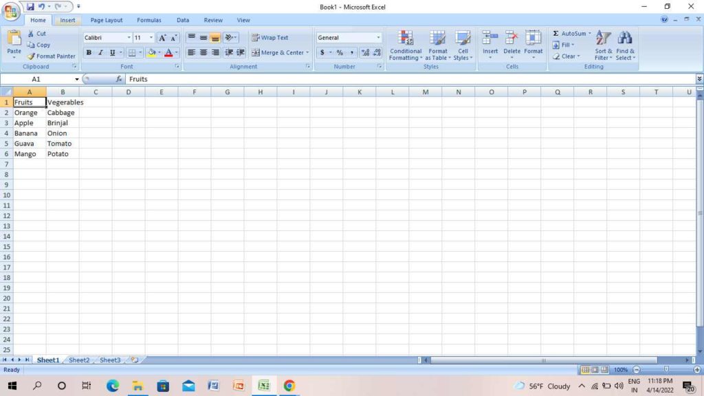
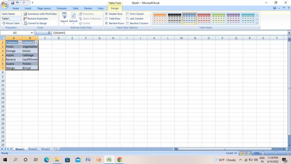
Slicers in Microsoft Excel is an amazing tool that can help you to sort the information for yourself as well as for others who open the Excel sheet. For example, you have made a table that consists of fruits and vegetables, and slicers show on the Excel sheet where the fruits are on the table. If you want to create yourself in a practical mode, then get the information in the below subheadings that will help you how to create slicers in Microsoft Excel. Also, read How to Create a Professional Invoice in Excel?
How to Create Slicers in Microsoft Excel | Create an Excel Table or Pivot Table
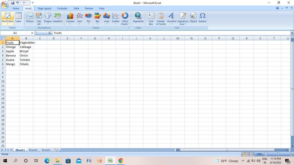
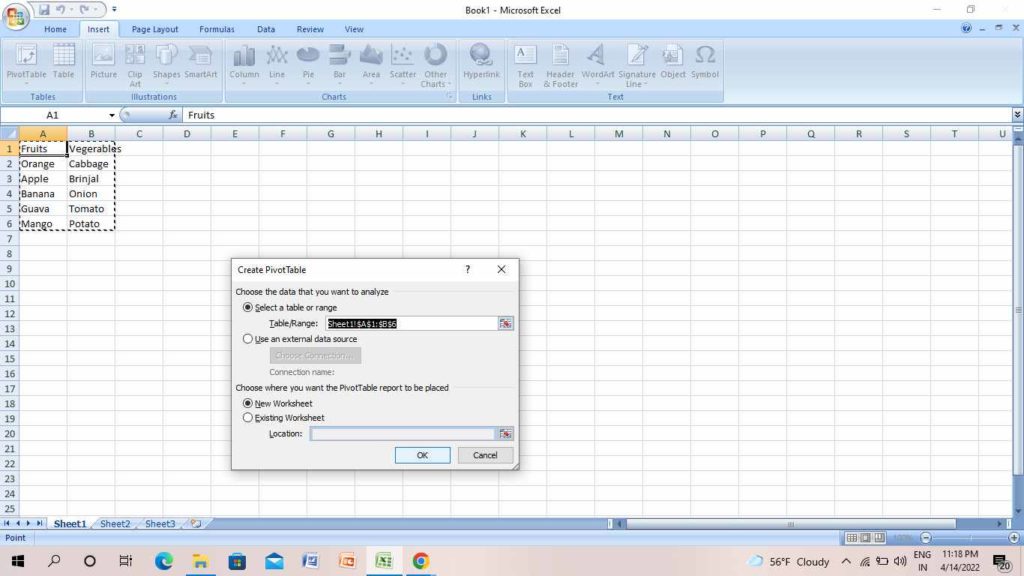
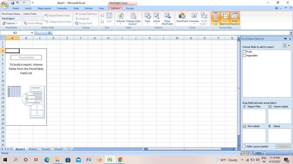
Before we begin to create Slicers in Microsoft Excel, you can convert the data into an Excel table or Pivot table. You can customize them accordingly as you want- Create a Pivot Table To create a Pivot table, follow the steps below- 3. Tap on Pivot Table. 4. On the Create Pivot Table Window, tap on Ok. 5. Pivot Table Field List will appear on the right side of the sheet. Select the data and drag them to different areas like Report Filter, Column Labels, Row Labels and Value. Thus, the Pivot data will be created for your data. Also, read How to Multiply Numbers in Excel: A Detailed Guide Create an Excel Table To create an Excel table, follow the steps below- Thus, the excel data will be created for your data. You can now easily create Slicers in Microsoft Excel for your Excel table data as well as for the Pivot table data.
How to Create Slicers in Microsoft Excel?
Once you got the idea of how to create an Excel table and Pivot data, now let’s move on to the next step. Here, you will learn how to create Slicers in Microsoft. Slicers are basically meant to filter the data visually. Slicers work faster and filter out the data of Pivot table, Excel table, Pivot Chart, or cube functions. To know more about it, follow the steps below- 3. Tap on Slicer. 4. On the insert slicers page, select the options. 5. Tap on Ok. Thus, the slicers will appear on the screen of your Excel sheet. You can now filter out the important information without affecting your actual data. Also, read How to Divide Numbers in Excel: A Detailed Guide
How to Create Slicers in Microsoft Excel?
If you want to know how to create Slicers in Microsoft Excel, follow the step by step guide in the below video-
Wrapping Up
This was all about how to create slicers in Microsoft Excel. You can easily copy the data of slicers and transfer it to multiple tables. This eliminates the manually entered data method and gets your work done on time. Now, it is time for a wrap-up. Keep visiting Path of EX for all the trending stuff. Stay tuned!
Δ